Conditional Formatting of EVOLVE grids
![]() Updated 2 years ago
by
Kerry Poe
Updated 2 years ago
by
Kerry Poe
Conditional Formatting
Conditional formatting can quickly identify critical information by creating rules that visually transform the appearance of the cell, text, or row based on the cell's value or formula to determine a value.
- Analyze all column cell values and visualize data distribution.
- Highlight specific values and dates.
- Highlight cells with the smallest or largest values.
- Highlight values below or above an average.
- Highlight unique or duplicate values.
- Use a custom formula to apply a color to specific cells.
- Temporarily highlight cells when their values change.
To apply Conditional Formatting
From an EVOLVE grid, right-click the desired column header and hover on Conditional Formatting to see the available options.
NOTE: the displayed options depend on the data type and may vary from column to column.
The initial options are predefined rule sets that will cover most formatting needs and may be a good starting point to test certain formatting conditions and see how the feature works. A value, range, custom condition, and formatting options may be specified for most of the available selections. Additionally, rules may be used in conjunction with other rules to help identify trends and patterns within the data. However, the true power of conditional formatting is realized in the Rules Manager when a formula is used to determine the formatting.
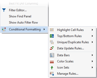

Predefined Formatting Conditions
Highlight Cell Rules
Used to highlight cells with the below comparison operators.
- Greater Than
- Cells in the column with a value above the specified value are highlighted.
- Less Than
- Cells in the column with a value below the specified value are highlighted.
- Between
- Cells in the column that fall within the specified range are highlighted.
- Equal To
- Cells in the column that match the specified value are highlighted.
- Text that contains
- Cells containing the specified value are highlighted.
- Custom Condition
- Cells adhering to one or many AND/OR conditions are highlighted.

Top/Bottom Rules
Used to highlight cells containing numerical values with the below comparison operators.
- Top 10 Items
- Based on a user-specified value, this option highlights the cells containing the largest values.
- Top 10%
- Based on a user-specified percentage, this option highlights the cells that fall into the specified percentile.
- Bottom 10 Items
- Based on a user-specified value, this option highlights the cells containing the smallest values.
- Bottom 10%
- Based on a user-specified percentage, this option highlights the cells that fall into the specified percentile.
- Above Average
- The average for all cells in the column is calculated, then all cells greater than the average value are highlighted.
- Below Average
- The average for all cells in the column is calculated, then all cells less than the average value are highlighted.

Unique/Duplicate Rules
- Unique Values
- Highlights a cell if its value does not match the values in other cells within the column.
- Duplicate Values
- Highlights cell with identical values.

Data Update Rules
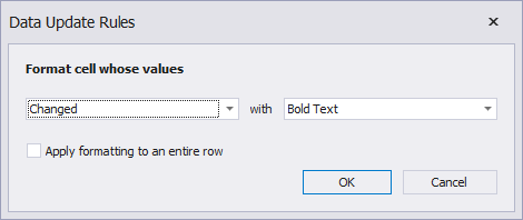
Used to highlight cells when the cell's value is:
- Changed
- Increased
- Decreased

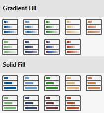
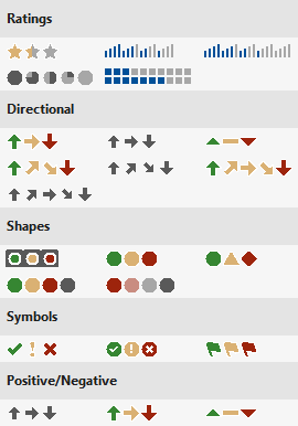
Data Bars
The Data Bars option partially fills cells with the selected color. The fill percentage depends on how small or large the cell value is compared to other values in this column. A vertical axis may be drawn at the zero value. In this instance, data bars for positive and negative values are displayed in opposite directions and are painted with different colors.

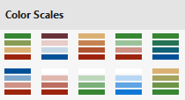
Color Scales
The Color Scales option compares cell values and fills these cells with solid colors chosen from a palette. The palette gradually shifts through two or three threshold colors.

Icon Sets
The Icon Sets option labels each value range with a corresponding icon.

Manage Rules
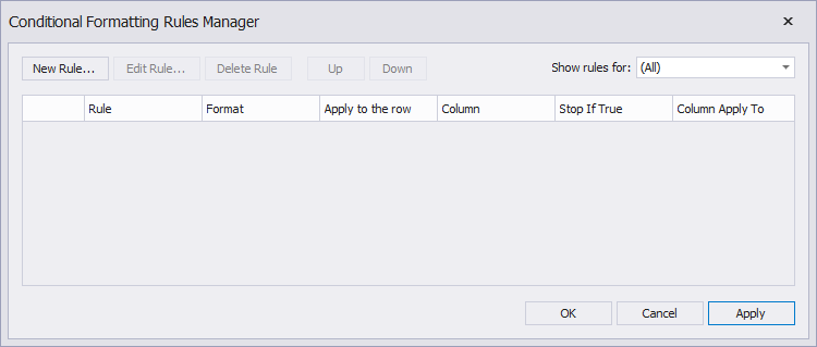
Overview of the Rules Manager
- New Rule button - creates a conditional formatting rule.
- Edit Rule button - modifies an existing conditional formatting rule.
- Delete Rule button - removes an existing conditional formatting rule.
- Up button - defines the rule's execution location in the grid.
- Down button - defines the rule's execution location in the grid.
- Show rules for menu - displays a list of available column headers and controls which rule sets are displayed in the grid.

Columns for the Rules Manager grid
- Selection checkbox - used to select a rule set.
- Rule - displays the rule name.
- Format - displays the selected format type.
- Apply to the row - boolean denoting whether only the cell or entire row is highlighted when the rule is true.
- Column - displays the column the rule is associated with.
- Stop If True - when selected, rule sets appearing lower in the list are not executed.
- Column Apply To - when defined, corresponding cells in the selected column are highlighted.

Using a formula when creating a new rule
- From the Conditional Formatting Rules Manager window, click New Rule.
- From the New Formatting Rule window, click Use a formula to determine which cells to format. The Edit the Rule Description panel is displayed.
- From the Edit the Rule Description panel, specify at least one condition and click Format.
- From the Format Cells window, choose the desired options from the Font and Fill tabs or select a predefined option from the Predefined Appearance tab.
- Once all elections have been made, click OK to close the Format Cells window.
- From the New Formatting Rule window, click OK.
- From the Conditional Formatting Rules Manager window, click Apply and/or OK.
